The VLOOKUP function is useful when a looking for information in a range. In its simplest wasy the forma is:
=VLOOKUP(lookup value, range that contans the look value, column number that contains the return value)
In this example, given the name of the product we want to return the product code. The first column must contain this data (product name), also the column values must be ordered from smallest to largest
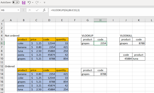
We can see what happens if they are not ordered, the top example returns the wrong codes for "grapes" while the lower example, which values are ordered returns the correct code.
The VLOOKALL function doesnt have these limitations, the lookup value can be in any column, and the values can be unordered. The format is:
VLOOKALL(range that contains the lookup value, column number that contains the lookup value, column value that contains the return value).
In this case the lookup value is "grapes" (J6), that value will be search in the column 1, while the code product is in column 3, the range for the search is B6:E10. So the formula would like this way (cell K6):
VLOOKALL(B6:E10,J6,1,3).
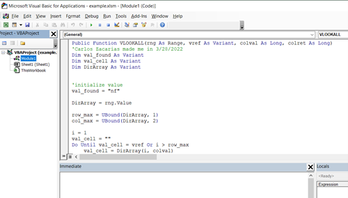
Below is the code to create this function. The workbook needs to be saved as xlsm, and a function module should be added to include a public function (insert → Module).